Microsoft Excel is a powerful tool for data analysis and reporting. It has over 475 formulas in its Functions Library. However, we have selected the most popular ones that everyone should know. Today we will share 10 frequently used function formulas. It is recommended that you should save them if you work with Exel frequently.
Excel Formulas
1. SUM
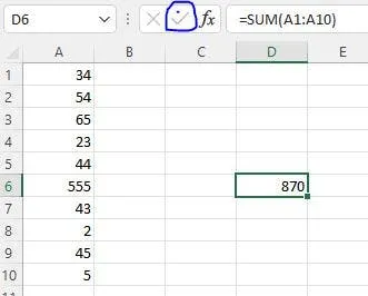
The SUM formula adds the values in a range of cells. To use the SUM formula, select the cell where you want the result to appear and type "=SUM(" followed by the range of cells you want to add, separated by commas. For example, "=SUM(A1:A10)" will add the values in cells A1 through A10. You may have to click on the tick circled in blue in the image below after writing the formula.

2. AVERAGE
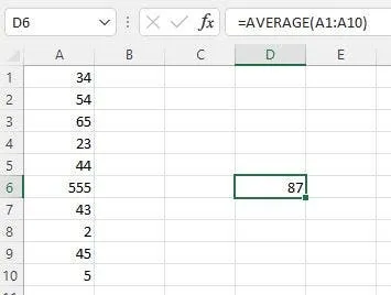
The AVERAGE formula calculates the average of the values in a range of cells. To use the AVERAGE formula, select the cell where you want the result to appear and type "=AVERAGE(" followed by the range of cells you want to average, separated by commas. For example, "=AVERAGE(A1:A10)" will calculate the average of the values in cells A1 through A10.

3. COUNT
The COUNT formula counts the number of cells in a range that contain numbers. To use the COUNT formula, select the cell where you want the result to appear and type "=COUNT(" followed by the range of cells you want to count, separated by commas. For example, "=COUNT(A1:A10)" will count the number of cells in cells A1 through A10 that contain numbers.
4. IF
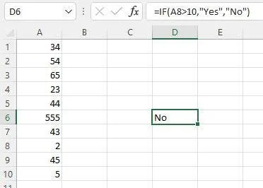
The IF formula tests a condition and returns one value if the condition is true and another value if the condition is false. To use the IF formula, select the cell where you want the result to appear and type "=IF(" followed by the condition you want to test, followed by the value to return if the condition is true, followed by the value to return if the condition is false. For example, "=IF(A1>10,"Yes","No")" will test if the value in cell A1 is greater than 10 and return "Yes" if it is true and "No" if it is false.

5. VLOOKUP
The VLOOKUP formula searches for a value in the first column of a table and returns a value in the same row from a specified column. To use the VLOOKUP formula, select the cell where you want the result to appear and type "=VLOOKUP(" followed by the value you want to search for, followed by the range of cells that contains the table, followed by the column number of the value you want to return, followed by "FALSE" if you want an exact match or "TRUE" if you want an approximate match. For example, "=VLOOKUP(A1,B1:C10,2,FALSE)" will search for the value in cell A1 in the first column of the table in cells B1 through C10 and return the value in the second column of the same row.
6. CONCATENATE
The CONCATENATE formula combines two or more strings of text into one string. To use the CONCATENATE formula, select the cell where you want the result to appear and type "=CONCATENATE(" followed by the strings of text you want to combine, separated by commas. For example, "=CONCATENATE(A1," ", B1)" will combine the text in cell A1 and cell B1 with a space between them.
7. LEFT
The LEFT formula returns a specified number of characters from the beginning of a string of text. To use the LEFT formula, select the cell where you want the result to appear and type "=LEFT(" followed by the cell that contains the string of text, followed by the number of characters you want to return. For example, "=LEFT(A1,5)" will return the first five characters of the text in cell A1.
8. RIGHT
The RIGHT formula returns a specified number of characters from the end of a string of text. To use the RIGHT formula, select the cell where you want the result to appear and type "=RIGHT(" followed by the cell that contains the string of text, followed by the number of characters you want to return. For example, "=RIGHT(A1,5)" will return the last five characters of the text in cell A1.

9. LEN
The LEN formula returns the number of characters in a string of text. To use the LEN formula, select the cell where you want the result to appear and type "=LEN(" followed by the cell that contains the string of text. For example, "=LEN(A1)" will return the number of characters in the text in cell A1.
10. TRIM
The TRIM formula removes extra spaces from a string of text. To use the TRIM formula, select the cell where you want the result to appear and type "=TRIM(" followed by the cell that contains the string of text. For example, "=TRIM(A1)" will remove extra spaces from the text in cell A1.
Final Words
Microsoft Excel is a powerful tool for data analysis and reporting, and mastering its formulas is essential for anyone working with data. The top 10 frequently used Microsoft Excel formulas include SUM, AVERAGE, COUNT, IF, VLOOKUP, CONCATENATE, LEFT, RIGHT, LEN, and TRIM. These formulas can perform a wide range of calculations and data analysis tasks in Excel. While there are many more formulas available in Excel, these 10 formulas are a great starting point for anyone looking to improve their Excel skills. By using these formulas, you can save time and increase your productivity when working with data. These are the top 10 frequently used Microsoft Excel formulas. By mastering these formulas, you can perform a wide range of calculations and data analysis tasks in Excel.
Popular News
Latest News
Loading


